Quantize ONNX Models with ONNX Runtime

You can cut an ONNX model’s weight storage by up to 4x with INT8 quantization, but a smaller model does not always mean lower latency.

If I had to sum up this guide in a few lines, it’s this:

• I start by preparing the model with shape inference and graph cleanup.
• I use dynamic quantization when I want the simplest path and don’t have calibration data.
• I use static quantization when I do have sample inputs and want lower CPU inference overhead.
• Then I check 3 things before shipping: file size, latency, and output drift.

The big point is simple: pick the quantization method based on your model type, your data, and your hardware. Transformers and RNNs often do well with dynamic quantization. CNNs and latency-focused CPU setups often fit static quantization better. And if accuracy drops, I can leave sensitive nodes in FP32, use per-channel weights, or improve calibration samples.

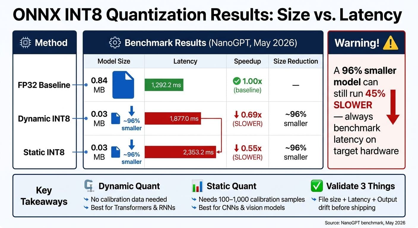
A key warning from the guide: in one May 2026 NanoGPT test, model size fell from 0.84 MB to 0.03 MB, but latency got worse - from 1,292.2 ms to 1,877.0 ms with dynamic INT8, and 2,353.2 ms with static INT8. So I don’t judge success by size alone.

Quick comparison

Method	Calibration data	Best fit	Main trade-off
Dynamic quantization	No	Transformers, RNNs, NLP models	Runtime activation scaling can add overhead
Static quantization	Yes	CNNs, vision models, CPU latency-focused use	Needs sample data and calibration setup

So if you want the short version: prepare the graph, quantize with the right flow, and test the result on the same hardware and inputs you plan to use.

Boost Your AI Models with INT8 Quantization 🚀 ONNX Static vs Dynamic + Python & C++ Speed Test

sbb-itb-903b5f2

Set Up the Environment and Preprocess the ONNX Model

Set up the environment before quantization so you don't run into version mismatches or preprocessing snags.

Install ONNX Runtime Quantization Dependencies

Install onnx and onnxruntime with pip:

pip install onnx onnxruntime

All quantization functions are part of the onnxruntime.quantization module, so you don't need a separate package. After that, make sure your Python version lines up with the onnxruntime build you installed, then do a quick import test:

import onnx
import onnxruntime
from onnxruntime.quantization import quantize_dynamic, quantize_static
print(onnxruntime.__version__)

If those imports run without errors, you're good to go.

Next up: get the model into shape so quantization runs against a clean graph.

Run Shape Inference and Model Optimization First

Run shape inference and optimization before quantization. A practical order looks like this:

• symbolic shape inference
• ONNX shape inference
• model optimization

Shape inference makes tensor shapes explicit in the graph. That helps the quantization tool map tensor shapes the right way.

Optimization matters too. Fused kernels, such as Linear + Bias + LayerNorm or Linear + ReLU, cut memory traffic and trim extra dequantize/requantize steps.

That usually makes the quantization step more dependable and makes the output easier to check.

Check Model and Hardware Constraints

A few checks up front can save you from painful debugging later.

First, make sure your model uses a supported opset version. If the model is large enough to go past standard ONNX file limits, use external data storage so quantization doesn't fail.

If you're targeting CPUs that don't have modern integer acceleration, use the reduce_range option to lower overflow risk. For accuracy, per-channel quantization is often the better call, especially for attention-heavy models. It uses a separate scale factor for each output channel, which keeps more of the original weight distribution intact.

With the model prepared, you can move on to dynamic or static quantization and run the matching command.

Apply Dynamic and Static Quantization Step by Step

Dynamic Quantization with quantize_dynamic

With the model preprocessed, the first move is usually simple: quantize the weights and check the INT8 output. Dynamic quantization is the calibration-free starting point. It pre-quantizes weights, then computes activation scales at inference time. That means no calibration data is needed, and it usually works well for Transformer and RNN models.

Here’s a minimal working example:

from onnxruntime.quantization import quantize_dynamic, QuantType

quantize_dynamic(
    model_input="model.onnx",
    model_output="model_dynamic_int8.onnx",
    weight_type=QuantType.QInt8,
    per_channel=True,
    reduce_range=False
)

weight_type=QuantType.QInt8 is the standard pick for CPU deployments. It can cut model size by up to 4x while keeping inference speed in a good place. Set per_channel=True for Transformer attention layers when you want better accuracy. It uses separate scales for each output channel, which usually keeps accuracy closer to the FP32 model than a single per-tensor scale.

If this baseline doesn’t give you the accuracy or speed you need, the next step is static quantization with calibration data.

Static Quantization with quantize_static and Calibration Data

Static quantization uses the same prepared model, but now you pass representative samples through a CalibrationDataReader. The goal is to precompute activation ranges from real inputs instead of estimating them at runtime.

You need to implement a CalibrationDataReader to supply those samples:

import numpy as np
from onnxruntime.quantization import CalibrationDataReader

class MyCalibReader(CalibrationDataReader):
    def __init__(self, data):
        self.data = iter(data)

    def get_next(self):
        try:
            return next(self.data)
        except StopIteration:
            return None

A good target is 100–1,000 representative samples that match your production inputs as closely as possible. For vision models, use images from the same domain you expect in production. For NLP models, use real text sequences, not dummy placeholder strings. Garbage in, garbage out applies here.

Once the reader is ready, call quantize_static with the calibration method you want:

from onnxruntime.quantization import quantize_static, CalibrationMethod, QuantFormat

quantize_static(
    model_input="model_preprocessed.onnx",
    model_output="model_static_int8.onnx",
    calibration_data_reader=MyCalibReader(samples),
    calibrate_method=CalibrationMethod.Entropy,
    quant_format=QuantFormat.QDQ
)

The main calibration methods differ in how they set activation ranges:

• MinMax uses the absolute minimum and maximum values.
• Entropy uses KL divergence to reduce information loss between the original and quantized distributions.
• Percentile clips outliers at a set threshold, such as 99.9%, which can help when activations have heavy tails.

For graph format, QDQ inserts QuantizeLinear and DequantizeLinear node pairs into the graph. It’s often the easier option when you need to inspect or debug the model. QOperator swaps original ops for quantized versions such as QLinearConv. Use QOperator only if your backend clearly supports it.

Key Command Options and When to Use Them

These options let you tune accuracy, compatibility, and graph format without changing the basic workflow:

Option	What it changes	When to use it	Main trade-off
per_channel	Per-output-channel weight scales for better accuracy.	For better accuracy on Transformer and CNN weights.	Different performance or compatibility.
reduce_range	Uses a narrower INT8 range for older CPUs or unstable accuracy.	On older CPUs or when accuracy is unstable.	May reduce peak speed or compression benefit.
weight_type	Sets the weight quantization type.	To choose 8-bit weight quantization for dynamic or static flows.	Affects model size, kernel support, and possible accuracy drift.
nodes_to_quantize	Quantizes only selected nodes.	When testing targeted quantization or protecting sensitive graph parts.	More control, but less overall size or speed gain.
nodes_to_exclude	Leaves selected nodes in higher precision.	When a few layers cause most of the accuracy loss.	Helps preserve accuracy, but reduces full-model optimization.
quant_format	Chooses QDQ or QOperator graph style.	Use QDQ for easier debugging; use QOperator only when your backend supports it explicitly.	Affects graph structure, compatibility, and sometimes performance.

Measure Size, Speed, and Output Drift After Quantization

Compare Model File Size

After quantization, test the model on the same hardware and with the same inputs you expect to use in production. Then compare the original and quantized .onnx files on disk with Python's os.path.getsize():

import os

fp32_size = os.path.getsize("model.onnx") / (1024 ** 2)
int8_size = os.path.getsize("model_dynamic_int8.onnx") / (1024 ** 2)
reduction = (fp32_size - int8_size) / fp32_size * 100

print(f"FP32: {fp32_size:.2f} MB | INT8: {int8_size:.2f} MB | Reduction: {reduction:.1f}%")

It helps to report both numbers: the file size in MB and the percentage drop. That way, you can tell at a glance whether the smaller model fits your deployment limits.

Benchmark Inference Latency and Throughput

A smaller file doesn't always mean a faster model. File size tells you about storage. Latency tells you what happens when the model actually runs.

Use time.perf_counter() for timing, and warm up the session first so startup work doesn't skew the numbers. Swap in your model's real input shape and dtype here:

import time
import numpy as np
import onnxruntime as ort

session = ort.InferenceSession("model_dynamic_int8.onnx")
input_name = session.get_inputs()[0].name
# Replace shape and dtype with your model's actual input
dummy_input = {input_name: np.zeros((batch_size, seq_len), dtype=input_dtype)}

# Warm-up
for _ in range(5):
    session.run(None, dummy_input)

# Timed runs
times = []
for _ in range(50):
    start = time.perf_counter()
    session.run(None, dummy_input)
    times.append((time.perf_counter() - start) * 1000)

print(f"Avg latency: {sum(times) / len(times):.2f} ms")

When you compare models, keep the setup the same. Same machine. Same input shape. Same runtime path. For example, if the quantized model runs with CPU INT8 kernels, the FP32 baseline should also be measured on CPU. If you're tracking throughput too, report tokens or samples per second using that same fixed input shape and hardware setup.

And here's the part that trips people up: quantization can shrink a model and still make it slower.

In a May 2026 benchmark of a 210,000-parameter NanoGPT model, dynamic INT8 quantization cut model size from 0.84 MB to 0.03 MB, but latency went up from 1,292.2 ms to 1,877.0 ms.

Method	Size (MB)	Latency (ms)	Speedup
FP32 (Baseline)	0.84	1,292.2	1.00x
Dynamic INT8	0.03	1,877.0	0.69x
Static INT8	0.03	2,353.2	0.55x

(Source:)

Check Output Drift and Fix Accuracy Loss

Size and latency only matter if the quantized model still stays close to the FP32 baseline. Run the same evaluation set through both models and compare logits or task metrics.

If the drift is too high, tweak the quantization setup. In many cases, it helps to:

• skip sensitive nodes like LayerNorm and embedding tables
• try static quantization again with representative calibration data
• switch to per-channel weights

That kind of tuning can make the difference between a tiny model that's usable and one that falls apart under test.

Conclusion: Pick the Right Quantization Flow and Validate the Result

Choosing between dynamic and static quantization comes down to two things: the data you have and the goal you're chasing. If you don't have a representative calibration dataset, dynamic quantization is the fastest path to a usable INT8 model. If you do have that data and runtime throughput is the priority, static quantization is the better choice because it precomputes scales and removes runtime activation scaling. Pick the flow that fits, then test it on the workload you actually care about.

A smaller INT8 model can still run slower. That's why you need to measure performance on your target hardware, not just assume the size drop will translate into better speed.

The bottleneck matters too. Memory-bound models usually gain the most from smaller weights. Compute-bound models may not see the same kind of lift.

In practice, the sequence is pretty simple: preprocess, quantize, validate. The workflow stays the same across models - run shape inference and optimization first, apply the right quantization flow, then measure size, latency, and output drift before shipping.

If the result misses the mark, tweak per-channel settings, adjust calibration data, or keep sensitive layers in FP32.

FAQs

How do I choose between dynamic and static quantization?

Dynamic quantization calculates activation parameters during inference. That makes it a good fit for NLP and Transformer models, where input lengths can change from one request to the next. It’s also easier to set up because it doesn’t need calibration data.

Static quantization computes those parameters ahead of time from a calibration dataset. It’s often the better pick for vision models like CNNs because it cuts runtime overhead and can improve performance. The tradeoff is setup: it takes more work to configure.

Why can an INT8 ONNX model be smaller but slower?

An INT8 model can take up less space and still run slower. That sounds backwards at first, but it happens all the time.

Here’s why: quantization cuts model size, not speed by default.

Faster inference depends on whether the hardware can run INT8 instructions well. On x86 CPUs, that often means support like VNNI. On GPUs, it can mean Tensor Cores. If that native support isn’t there, the runtime may need to do extra work behind the scenes.

That extra work can include:

• Format conversions
• Extra memory movement
• Other runtime overhead

And once that happens, latency can go up instead of down.

What should I do if quantization hurts accuracy?

First, compare the float32 and quantized models with the qdq_loss_debug module to find the layers behind the accuracy drop.

Then calibrate with a representative dataset of at least 500 samples. From there, you can try:

• QAT to train the model with quantization in the loop
• Distillation to help the quantized model stay closer to the float32 model
• Selective higher-precision fallbacks for the nodes that are causing the most damage

That gives you a clean path: find the weak spots first, then fix ONLY the parts that need attention.